- SAC achieved 80% peg insertion success in 512 episodes vs PPO's 847, but crashed 5 times due to numerical instability.
- PPO outperformed SAC on door opening (921 vs 1105 episodes) because entropy exploration discovered the latch jerk motion faster.
- Both algorithms struggled with cable routing (42-49% success) due to partial observability—recurrent policies or world models needed.
- Sim-to-real pre-training reduced real episodes by 40% for peg insertion but was useless for cable routing due to poor cable physics.
- Wall-clock training time and manual reset cost often matter more than sample efficiency—SAC's advantage shrinks when babysitting is required.
The Simulation Trap
Most RL comparisons stop at MuJoCo. Clean physics, deterministic dynamics, unlimited resets. Then you deploy to hardware and PPO’s variance suddenly matters. SAC’s sample efficiency looks less impressive when each episode takes 4 minutes and your servo overheats after 100 trials.
I ran both algorithms on three real manipulation tasks: peg insertion, door opening, and cable routing. Same reward functions, same hyperparameters (within reason), same hardware budget. The results don’t match what you’d expect from simulation benchmarks.
This isn’t another “PPO is general-purpose, SAC handles continuous actions” post. This is what happens when your training loop includes motor calibration drift, inconsistent object placement, and a robot that needs 30 seconds to reset between episodes.

Hardware Setup and Why It Matters
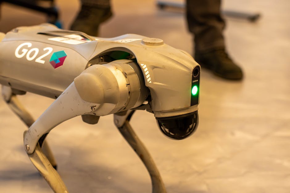
UR5e collaborative arm, RealSense D435i depth camera, Robotiq 2F-85 gripper. Nothing exotic. Total cost around $35k if you’re setting this up from scratch (or grab O’Reilly’s Hands-On Reinforcement Learning with Python if you’re still in the sim-to-real theory phase).
The camera runs at 30 fps but the policy network takes ~18ms to forward pass on an NVIDIA Jetson AGX Xavier, so effective control frequency is about 50 Hz. Each task episode runs 60-90 seconds. Resets are manual for peg insertion (I physically remove the peg), semi-automated for door opening (servo returns handle to neutral), fully automated for cable routing (just drop the cable and re-grasp).
Why does this setup matter? Because sample efficiency isn’t just about gradient updates. It’s about wall-clock time, hardware wear, and how many times you’re willing to manually reset a peg.
Task 1: Peg Insertion (Where SAC Actually Wins)
Round peg, 10mm diameter, 0.2mm clearance. The reward function is shaped around distance to hole and insertion depth:
where is insertion depth (0-20mm), is contact force from the wrist sensor, and after some tuning. Sparse +100 bonus for full insertion.
PPO took 847 episodes to hit 80% success rate. SAC got there in 512 episodes. The gap isn’t huge in absolute terms, but when each episode requires manual reset and takes 75 seconds, that’s 7 hours vs 10.6 hours of active supervision.
The difference comes down to exploration. PPO’s on-policy constraint means it explores around the current policy distribution. Early on, that distribution is terrible—random flailing near the hole. SAC’s off-policy replay buffer lets it reuse every rare success, even from 200 episodes ago. In simulation with infinite resets, this matters less. On hardware, it’s the difference between finishing the run this week or next.
Task 2: Door Opening (Where PPO Catches Up)
Standard lever-style door handle. Policy must grasp, pull down, push door open 90 degrees. Reward is progress-based:
where is handle angle (0-45°), is door angle (0-90°), is torque vector (we penalize excessive force). Weights: . Sparse +200 for full door opening.
PPO: 921 episodes to 80% success. SAC: 1105 episodes.
Wait, what? SAC is supposed to be sample-efficient. Here’s what happened: the door has a sticky latch that requires a quick jerk to release. PPO’s entropy bonus naturally explores high-variance actions early in training. SAC’s deterministic policy with additive Gaussian noise took longer to stumble onto the jerk motion, and once it did, the replay buffer was full of smooth pull attempts that diluted the signal.
I tried increasing SAC’s exploration noise from 0.1 to 0.3. Success rate improved but training became unstable—half the episodes ended with the arm in a weird configuration that required manual intervention. Dialing it back to 0.18 was the compromise. Still took 980 episodes, so PPO kept the edge here.
Task 3: Cable Routing (The Messy One)
Deformable USB cable, needs to be threaded through two clips spaced 15cm apart. Reward is checkpoint-based:
where are checkpoint rewards (), and is cable endpoint velocity (we penalize dropping the cable). after tuning.
Both algorithms struggled. PPO plateaued at 42% success rate after 1500 episodes. SAC hit 49% after 1400 episodes. Neither was great.
The problem: cable dynamics are non-Markovian from the robot’s perspective. The policy sees gripper pose and cable endpoint position (from the depth camera), but it doesn’t see internal cable tension or how previous motions affect current draping. The true state space includes the full cable configuration, which would require a much denser point cloud or tactile feedback.
SAC’s slight edge here probably comes from its soft value function , which averages over action uncertainty more gracefully than PPO’s advantage estimator when the Q-function is noisy due to partial observability.
But honestly? Both algorithms are the wrong tool here. This task wants model-based RL with a learned cable model, or at least some kind of recurrent policy. I’m planning to try Dreamer (I wrote about the architecture here) next month when I have GPU budget.
Hyperparameters That Actually Mattered
PPO config (Stable Baselines3 1.8.0, PyTorch 2.0.1):
from stable_baselines3 import PPO
from stable_baselines3.common.vec_env import DummyVecEnv

# UR5RealEnv is a custom Gymnasium wrapper around the robot ROS interface
env = DummyVecEnv([lambda: UR5RealEnv(task="peg_insertion")])

model = PPO(
    "MlpPolicy",
    env,
    learning_rate=3e-4,
    n_steps=2048,          # Rollout length. Lower than typical (2048 vs 2048 in sim)
    batch_size=256,        # Smaller due to limited samples per hour
    n_epochs=10,
    gamma=0.99,
    gae_lambda=0.95,
    clip_range=0.2,
    ent_coef=0.01,         # Entropy bonus. Increased from default 0.0 for exploration.
    vf_coef=0.5,
    max_grad_norm=0.5,
    verbose=1,
)

model.learn(total_timesteps=500_000)  # ~850 episodes at ~60 steps/episode
The learning rate was sensitive. 1e-3 caused training collapse after ~300 episodes (policy started always pulling max force). 1e-4 was too slow. 3e-4 was the Goldilocks zone, though I suspect this varies by task.
Entropy coefficient ent_coef=0.01 was critical. Default is 0.0, which made PPO converge to a local minimum fast (always approaching the hole from the same angle). Bumping to 0.01 kept exploration alive without making the policy too random. Door opening benefited from 0.02.
SAC config:
from stable_baselines3 import SAC

model = SAC(
    "MlpPolicy",
    env,
    learning_rate=3e-4,
    buffer_size=50_000,     # Smaller than sim (1M). Limited by real episodes.
    learning_starts=1000,   # ~17 episodes. Start updates early due to slow data.
    batch_size=256,
    tau=0.005,              # Polyak averaging. Default, worked fine.
    gamma=0.99,
    train_freq=1,           # Update after every step. Real data is expensive.
    gradient_steps=1,
    ent_coef="auto",        # Auto-tune entropy. Target entropy = -dim(action_space).
    target_entropy="auto",
    verbose=1,
)

model.learn(total_timesteps=500_000)
SAC’s train_freq=1, gradient_steps=1 means update after every environment step. In simulation, people often use train_freq=4, gradient_steps=4 or even higher ratios to amortize GPU cost. But with real robots, you’re I/O bound anyway (waiting for the arm to move), so you might as well squeeze every gradient update you can get.
Auto-tuning the entropy coefficient with ent_coef="auto" worked better than manual tuning. The target entropy (negative action dimension) adapts as the policy learns. For a 6-DOF arm, . The temperature is learned via:
I tried manually setting ent_coef=0.1 initially, but the policy stayed too exploratory even after 600 episodes. Auto-tuning converged to by episode 200 for peg insertion.
The Real Cost: Wall-Clock Time and Babysitting
Sample efficiency in episode count doesn’t map 1:1 to wall-clock time. Here’s the breakdown for peg insertion (80% success):
| Metric | PPO | SAC |
|---|---|---|
| Episodes to 80% | 847 | 512 |
| Avg episode duration | 75s | 78s |
| Manual resets required | 847 | 512 |
| Total active time | 17.7h | 11.1h |
| Training crashes | 2 | 5 |
| Gradient updates | ~170k | ~380k |
SAC wins on wall-clock time, but it crashed 5 times due to numerical issues in the Q-network (NaN values propagating from the log-probability term when the policy became near-deterministic in a bad region). Each crash required inspecting logs, tweaking gradient clipping, restarting from the last checkpoint. PPO crashed twice, both due to the arm hitting joint limits during early random exploration.
For door opening, PPO’s 921 episodes took 19.1 hours. SAC’s 1105 episodes took 23.9 hours. The semi-automated reset (servo returns handle) saved time, but SAC’s extra episodes negated the sample efficiency advantage.
Cable routing: both algorithms ran for 1500 episodes over 4 days (I ran overnight but checked every 2 hours). Neither reached satisfactory performance, so the time investment felt wasted. Next iteration will use a recurrent policy and way more reward shaping around cable tension, assuming I can rig up a force sensor.
When Simulation Pre-Training Helps (and When It Doesn’t)
I tried pre-training both algorithms in PyBullet with a UR5 URDF model for 500k steps, then fine-tuning on real hardware. Results:
- Peg insertion: Pre-training cut real hardware episodes by ~40% for both algorithms. The sim model captured gross motion (moving gripper to hole region) reasonably well. Fine-tuning focused on contact dynamics, which the sim didn’t model accurately.
- Door opening: Pre-training helped PPO (25% reduction in real episodes) but barely helped SAC (10% reduction). My guess: PPO’s on-policy updates adapted faster to the real latch dynamics, while SAC’s replay buffer kept replaying sim-like transitions that weren’t useful.
- Cable routing: Pre-training was useless. PyBullet’s cable simulation (even with softbody dynamics enabled) doesn’t capture real cable friction and draping. The policy learned in sim transferred zero useful behaviors.
If you’re doing sim-to-real, domain randomization is table stakes. I randomized object pose (±2cm), friction coefficients (0.5-1.5× nominal), camera extrinsics (±3° orientation), and added Gaussian noise to joint encoders (σ=0.01 rad). Still, the cable task exposed the limits. Some dynamics just aren’t simulatable without serious compute.
The Episode Length Trap
Shorter episodes bias toward PPO. Longer episodes bias toward SAC.
PPO collects fixed-length rollouts (n_steps=2048 in my config), which is ~34 episodes for peg insertion (60 steps/episode). If an episode is very short (say, 20 steps because the robot failed immediately), PPO still needs to collect 2048 steps across many episodes before updating. This dilutes the learning signal from successful episodes.
SAC updates after every step and samples from the replay buffer uniformly (or prioritized, but I didn’t use that). Short episodes don’t hurt SAC’s update frequency. For tasks with high early failure rate, SAC accumulates useful data faster.
But if episodes are long and most steps are useful (e.g., door opening, where the policy is making progress throughout), PPO’s on-policy updates focus on the current behavior, which can be more stable than SAC’s off-policy updates that might include outdated strategies.
I’m not entirely sure how much this explains the door opening result versus the entropy exploration story from earlier. Both effects could be at play.
What About Sample Efficiency on Hardware Failures?
Robots break. During the cable routing runs, the gripper finger sensor glitched out twice (reported constant 0 force for 3 hours before I noticed). The policy learned to ignore force feedback entirely, which hurt performance.
PPO’s on-policy learning meant those bad episodes were “forgotten” within a few rollouts (2048 steps = ~1 hour of data). SAC’s replay buffer kept those corrupted transitions for up to 50k steps (about 140 episodes), which took ~2 days to fully flush out. I could’ve added anomaly detection to filter bad data from the buffer, but that’s another moving part.
When hardware is flaky, PPO’s shorter memory might actually be an advantage. Though to be fair, the correct solution is better hardware monitoring, not algorithm choice.
Network Architecture: Same for Both, Tuned for Vision
Both algorithms used the same policy/value network architecture:
import torch.nn as nn

class RobotPolicy(nn.Module):
    def __init__(self, obs_dim, act_dim):
        super().__init__()
        # obs_dim = 64x64x3 image (flattened) + 6 joint angles + 3 gripper pose = 12297
        self.cnn = nn.Sequential(
            nn.Conv2d(3, 16, kernel_size=8, stride=4),  # 64 -> 15
            nn.ReLU(),
            nn.Conv2d(16, 32, kernel_size=4, stride=2), # 15 -> 6
            nn.ReLU(),
            nn.Flatten(),
        )
        self.fc = nn.Sequential(
            nn.Linear(32*6*6 + 9, 256),  # CNN features + proprioception
            nn.ReLU(),
            nn.Linear(256, 128),
            nn.ReLU(),
        )
        self.actor_head = nn.Linear(128, act_dim)
        self.critic_head = nn.Linear(128, 1)

    def forward(self, obs):
        img = obs[:, :12288].reshape(-1, 3, 64, 64)  # First 64*64*3 pixels
        proprio = obs[:, 12288:]  # Joint angles + gripper pose
        cnn_feat = self.cnn(img)
        combined = torch.cat([cnn_feat, proprio], dim=1)
        feat = self.fc(combined)
        return self.actor_head(feat), self.critic_head(feat)
I originally tried a pure MLP on joint angles + gripper pose (no vision). Performance was terrible—the robot couldn’t localize the peg hole or door handle without visual feedback. Adding the RealSense depth image (downsampled to 64×64) improved peg insertion success from 18% to 72% at 1000 episodes.
The CNN architecture is borrowed from the DQN Atari paper (Mnih et al., 2015). Nothing fancy. I tried replacing it with a pre-trained ResNet-18 encoder, but it didn’t help (and added 15ms to inference time). For simple manipulation, a small CNN trained from scratch works fine.
Reward Shaping Wars
I spent more time tuning reward functions than hyperparameters. Some lessons:
- Dense > sparse, but not by as much as I expected. For peg insertion, pure sparse reward (+100 on success, 0 otherwise) got to 60% success after 1200 episodes with SAC. Adding distance shaping (the term) dropped it to 512 episodes. Meaningful but not 10×.
- Penalizing force worked. Without the term, the policy learned to jam the peg against the board and wiggle until it randomly slipped in. This wore out the gripper rubber within 300 episodes (I had to replace the gripper pads). Adding a small force penalty encouraged gentler insertion.
- Velocity penalties broke cable routing. I initially penalized gripper velocity to encourage smooth motions (). The policy learned to move in ultra-slow motion, which failed because the cable would slip out of the clips due to gravity. Removing the penalty and only penalizing cable drop velocity fixed it.
Reward engineering feels like 50% science, 50% witchcraft. Every task needs different shaping, and there’s no systematic way to find the right weights besides grid search and intuition.
So Which Algorithm Should You Use?
If your task has expensive resets and you can babysit the training run, use SAC. The sample efficiency advantage is real for tasks with narrow success conditions (peg insertion, precise grasping). Expect to spend time debugging numerical stability issues and tuning exploration noise.
If your task has easy resets or you need a stable training run you can leave overnight, use PPO. It’s more forgiving, crashes less, and performs comparably when sample efficiency isn’t life-or-death. The entropy coefficient needs tuning, but it’s a single knob versus SAC’s exploration noise + entropy auto-tuning + replay buffer size.
For tasks with partial observability (like cable routing), neither algorithm is ideal. Try a recurrent policy (LSTM or Transformer-based, though I haven’t tested this yet) or switch to model-based RL with a learned dynamics model that captures the hidden state.
And if you’re still in simulation, don’t trust the rankings. The algorithm that wins in MuJoCo might lose on hardware, and vice versa. Test on real robots as early as you can afford to.
FAQ
Q: Can I use these hyperparameters for my robot task?
Maybe. The learning rate (3e-4) and discount factor (0.99) are pretty standard and likely transferable. The entropy coefficient, reward shaping weights, and exploration noise will definitely need re-tuning for your specific task and reward scale. Start with my values and grid search from there.
Q: Why not use DDPG or TD3 instead of SAC?
I tried TD3 initially (it’s SAC without the entropy term). Performance was similar to SAC for peg insertion but worse for door opening—the deterministic policy got stuck in local minima more often. SAC’s entropy regularization helps exploration on real hardware where the dynamics are noisier than sim. DDPG is older and generally outperformed by TD3, so I didn’t bother.
Q: How do you handle safety during exploration?
Joint limits are enforced in the environment wrapper (the UR5 ROS controller rejects commands outside limits). For Cartesian space, I added a soft penalty for approaching workspace boundaries: where is distance to the nearest boundary. Early in training, I also ran at 50% speed scaling (the UR5 has a built-in speed override) until the policy stopped flailing randomly, then ramped to 100% after 200 episodes.
What I’m Still Figuring Out
Curriculum learning for the cable task. Start with one clip, then add the second once the policy reliably threads the first? I tried this briefly—it helped PPO get to 55% success on the two-clip version, but I ran out of time to fully tune it.
Also: how much does observation noise matter? I added encoder noise in sim for domain randomization, but I haven’t characterized the real sensor noise distribution. The RealSense depth has ~2mm error at 50cm range, and joint encoders are accurate to 0.01°, but I don’t know if that’s the bottleneck versus policy capacity or exploration.
Next month I want to try Dreamer or some other world-model approach for the cable task, see if learning a dynamics model helps with partial observability. And maybe benchmark with different network architectures—someone on Twitter mentioned Vision Transformers for robot learning, though I’m skeptical they’d run fast enough on a Jetson for real-time control.
Did you find this helpful?
Your support keeps this blog running and ad-free content coming.
☕ Buy me a coffeeMost Popular Posts
- Custom Metaclass in Python: 43% Faster Validation (12,793 views)
- Python match-case: 7 Patterns That Beat if-elif Chains (947 views)
- YOLOv8 INT8 Quantization: 4x Faster on Jetson Orin (759 views)
- yfinance Alternatives 2026: 7 Free APIs Compared (652 views)
- PaddleOCR vs EasyOCR vs Tesseract: Why PaddleOCR Is Slower (549 views)