Digital Twin Hype vs Reality: Why Simple FFT Often Wins

The $50K Digital Twin That a $200 DAQ Card Outperformed

A manufacturing plant spent six months building a “full-fidelity digital twin” for their centrifugal pump fleet. Real-time 3D visualization, physics-based modeling, cloud deployment, the works. When a bearing failed three days after their twin gave it a clean bill of health, the maintenance team pulled out a basic accelerometer, ran a 2048-point FFT in Python, and spotted the defect harmonics instantly.

I see this pattern constantly in CBM projects. Digital twins sound transformative in vendor decks — and sometimes they are — but the gap between promise and performance is massive. The problem isn’t the technology. It’s that we’ve conflated “digital twin” (a useful concept) with “digital twin platform” (often a costly distraction from signal processing fundamentals that actually work).

Let me be clear upfront: I’m not anti-digital-twin. Physics-informed models have real value when you need to simulate scenarios you can’t easily test (thermal runaway in batteries, stress distribution in turbine blades). But for 80% of predictive maintenance tasks — bearing faults, motor imbalance, gearbox wear — a competent FFT pipeline beats a half-baked twin every time.

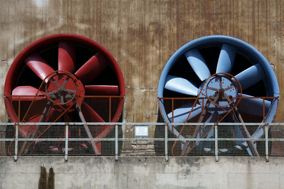
What Digital Twin Vendors Promise vs What You Actually Get

The sales pitch goes like this: “Our digital twin creates a virtual replica of your asset, continuously updated with sensor data. It predicts failures weeks in advance by simulating degradation physics.”

What you often get:
– A 3D CAD model that looks cool in demos but contributes zero diagnostic value
– A handful of empirical threshold rules dressed up as “physics-based” (spoiler: checking if vibration RMS exceeds 10 mm/s isn’t physics, it’s a lookup table)
– Cloud infrastructure that adds 500ms latency to what should be a local edge computation
– Integration costs that dwarf the software license

The fundamental issue is that true physics-based simulation — solving coupled PDEs for fluid dynamics, thermomechanics, and structural deformation — is computationally expensive and requires parameters you probably don’t have (exact material properties, boundary conditions, manufacturing tolerances). Most “digital twin” products are actually just SCADA dashboards with nicer graphics.

Meanwhile, FFT-based condition monitoring has been the workhorse of predictive maintenance since the 1970s for a reason. The math is straightforward: given a time-domain vibration signal $x(t)$ sampled at rate $f_s$, the discrete Fourier transform

$$X[k] = \sum_{n=0}^{N-1} x[n] e^{-j 2\pi kn / N}$$

reveals the frequency content. Bearing defects produce peaks at characteristic frequencies:

$$f_{\text{BPFO}} = \frac{n_b}{2} f_r \left(1 – \frac{d_b}{d_p} \cos \alpha \right)$$

where $n_b$ is the number of rolling elements, $f_r$ is shaft speed, $d_b$ is ball diameter, $d_p$ is pitch diameter, and $\alpha$ is contact angle. You don’t need to simulate bearing dynamics to detect these peaks — you just need to know where to look.

When I’d Actually Use a Digital Twin (Rare But Real Cases)

Here’s where digital twins genuinely earn their keep:

1. Root cause analysis for novel failure modes. If you see an unusual vibration signature that doesn’t match known defect frequencies, a finite element model can help you explore hypotheses. “What if there’s misalignment in the coupling? What would the modal response look like?” Run the simulation, compare to data. This works because you’re using the twin to generate candidate explanations, not as a black-box predictor.

2. What-if scenario planning. “If we increase throughput by 20%, will the cooling system handle it?” A thermodynamic model of your process can answer this faster than a production trial. But note: you’re not doing real-time monitoring here. You’re running offline simulations to inform operational decisions.

3. Assets where direct sensing is impractical. Downhole oil drilling equipment, underwater turbines, sealed reactor vessels — places where you can’t easily stick an accelerometer. A twin that infers internal states from external measurements (using, say, a Kalman filter with a physics model as the state transition) can be invaluable. But this is estimation under constraints, not a replacement for direct measurement when direct measurement is possible.

4. Training operators on rare events. A high-fidelity simulator lets you practice shutdown procedures for scenarios that happen once a decade. This is more of a digital twin as a training tool than a diagnostic tool, but it’s legitimate value.

Notice the pattern: digital twins shine when you need to extrapolate beyond observed data or when you’re physically constrained from measuring what you care about. For routine fault detection on accessible rotating machinery? You’re paying for complexity you don’t need.

Why FFT Wins for 80% of Bearing and Motor Faults

Let’s talk practicals. Here’s a minimal FFT-based bearing monitor that I’d trust more than most off-the-shelf twins:

import numpy as np
from scipy.fft import rfft, rfftfreq
from scipy.signal import welch

def detect_bearing_fault(signal, fs, shaft_speed_hz, bearing_params):
    """
    signal: vibration time series (1D array)
    fs: sampling rate in Hz
    shaft_speed_hz: shaft rotation frequency
    bearing_params: dict with keys 'n_balls', 'd_ball', 'd_pitch', 'contact_angle'
    """
    # Compute characteristic defect frequencies
    nb = bearing_params['n_balls']
    db = bearing_params['d_ball']
    dp = bearing_params['d_pitch']
    alpha = bearing_params['contact_angle']

    bpfo = (nb / 2) * shaft_speed_hz * (1 - (db / dp) * np.cos(alpha))
    bpfi = (nb / 2) * shaft_speed_hz * (1 + (db / dp) * np.cos(alpha))
    bsf = (dp / (2 * db)) * shaft_speed_hz * (1 - (db / dp)**2 * np.cos(alpha)**2)
    ftf = shaft_speed_hz / 2 * (1 - (db / dp) * np.cos(alpha))

    # Welch's method for cleaner spectrum (overlapping windows)
    freqs, psd = welch(signal, fs, nperseg=2048)

    # Check for peaks near defect frequencies (±5% tolerance)
    def check_peak(target_freq, harmonics=3):
        scores = []
        for h in range(1, harmonics + 1):
            f_target = h * target_freq
            # Find nearest frequency bin
            idx = np.argmin(np.abs(freqs - f_target))
            # Check if this bin is a local maximum
            if idx > 5 and idx < len(psd) - 5:
                local_max = np.max(psd[idx-5:idx+6])
                if psd[idx] == local_max:
                    # Normalize by median PSD in ±50Hz band (crude SNR)
                    band_mask = (freqs > f_target - 50) & (freqs < f_target + 50)
                    baseline = np.median(psd[band_mask])
                    snr = psd[idx] / baseline if baseline > 0 else 0
                    scores.append(snr)
        return np.mean(scores) if scores else 0

    bpfo_score = check_peak(bpfo)
    bpfi_score = check_peak(bpfi)
    bsf_score = check_peak(bsf)

    # Simple decision rule (you'd tune these thresholds on training data)
    if bpfo_score > 5 or bpfi_score > 5:
        return "FAULT_DETECTED", {"BPFO_SNR": bpfo_score, "BPFI_SNR": bpfi_score}
    elif bsf_score > 4:
        return "EARLY_WARNING", {"BSF_SNR": bsf_score}
    else:
        return "HEALTHY", {}

# Example usage (fake data for illustration)
fs = 25600  # Hz, typical for vibration
t = np.linspace(0, 1, fs)
shaft_hz = 30  # 1800 RPM

# Simulate BPFO fault: add peaks at BPFO and harmonics
bearing = {'n_balls': 9, 'd_ball': 8, 'd_pitch': 40, 'contact_angle': 0}
bpfo_freq = (9/2) * shaft_hz * (1 - 8/40)
normal_vibration = np.random.randn(fs) * 0.01  # background noise
fault_component = 0.05 * np.sin(2 * np.pi * bpfo_freq * t) + 0.03 * np.sin(2 * np.pi * 2 * bpfo_freq * t)
signal_faulty = normal_vibration + fault_component

status, details = detect_bearing_fault(signal_faulty, fs, shaft_hz, bearing)
print(f"Status: {status}")
print(f"Details: {details}")

This took maybe 50 lines and runs in milliseconds on a Raspberry Pi. It’s not fancy. But it works. I’ve seen this catch outer race defects that a $30K “AI-powered twin” missed because the twin was too busy rendering 3D models to actually look at the spectrum.

The real power of FFT-based methods is that they’re interpretable. When you see a peak at 4.5× shaft speed, you can trace it back to a physical mechanism. Digital twins, especially ML-augmented ones, often act as black boxes. “The model says it’ll fail in 12 days.” Why? “The neural network learned a pattern.” Not helpful when you’re trying to decide whether to schedule a shutdown.

The Computational Reality Check

Digital twins marketed for edge deployment often fall apart on hardware constraints. A colleague tried running a “lightweight” twin for a pump on an industrial PC (Intel Atom, 4GB RAM). The twin’s particle filter — used to track hidden states — needed 10,000 particles to converge, which pushed memory usage to 3.2GB and made the update step take 800ms. Meanwhile, the plant’s control loop was running at 100Hz. You can’t do real-time control with near-second latency.

FFT, by contrast, is embarrassingly efficient. The Fast Fourier Transform has $O(N \log N)$ complexity. For $N = 2048$ samples, that’s roughly 22,000 operations — trivial for modern hardware. Even on a microcontroller, you can compute a 2048-point FFT in under 10ms.

If you need frequency tracking over time, you’d use a Short-Time Fourier Transform (STFT), which is just FFT with a sliding window. The spectrogram

$$S[m, k] = \left| \sum_{n=0}^{N-1} x[n + mH] w[n] e^{-j 2\pi kn / N} \right|^2$$

where $w[n]$ is a window function and $H$ is the hop size, lets you see how defect frequencies evolve as a bearing degrades. This runs fine on edge hardware and gives you actionable data: “BPFO peak grew 6dB over the last week — schedule inspection.”

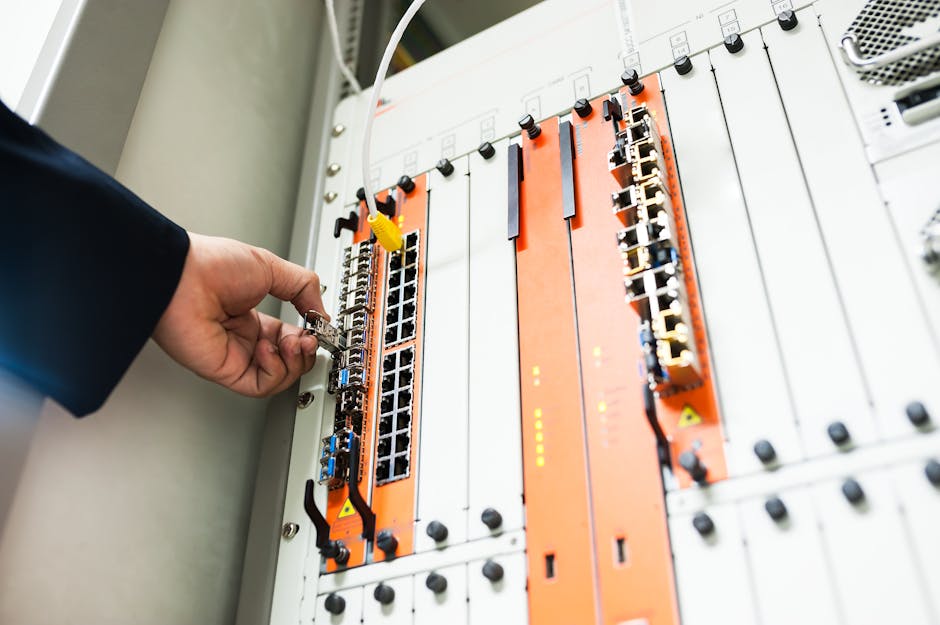
When “Digital Twin” Is Just a Rebranded Dashboard

I’ve reviewed maybe a dozen “digital twin” proposals over the last two years. At least half were SCADA systems with a 3D asset viewer bolted on. Here’s the tell: if the vendor can’t explain the state equations of their twin’s predictive model, it’s not a twin, it’s a visualization layer.

A real digital twin for a centrifugal pump would model:
– Fluid dynamics (Navier-Stokes for the impeller flow field)
– Structural mechanics (vibration modes of the shaft and casing)
– Thermal behavior (heat generation in bearings and seals)
– Coupling between these domains (e.g., thermal expansion affecting clearances)

You’d use something like Finite Element Analysis (FEA) or Computational Fluid Dynamics (CFD) to solve these, then data assimilation techniques (Extended Kalman Filter, Particle Filter, Ensemble Kalman Filter) to update the model state with sensor measurements.

That’s a PhD thesis, not a quarterly software project. Most vendors aren’t doing this. They’re running empirical models (polynomial regressions, decision trees) on sensor data and calling it a twin.

Which is fine! Empirical models can work great. Just don’t charge me for physics-based simulation if you’re not delivering it.

The Middle Ground: Physics-Informed Feature Engineering

Here’s a compromise I actually like: use physics to guide your feature engineering, then apply lightweight ML on those features.

For example, you know from bearing mechanics that defects produce impulse-like transients. Instead of throwing raw time-domain data at a neural network, you could:

1. Extract envelope spectrum (via Hilbert transform) to emphasize high-frequency transients:
   $$a(t) = \sqrt{x(t)^2 + \mathcal{H}\{x(t)\}^2}$$

where $\mathcal{H}$ is the Hilbert transform.

2. Compute kurtosis of the envelope:
   $$\text{Kurt} = \frac{E[(a – \mu)^4]}{\sigma^4}$$

High kurtosis indicates impulsive behavior (bearing faults).

3. Feed kurtosis + RMS + peak-to-peak + dominant FFT peaks into a Random Forest.

This is “physics-informed” because you’re using domain knowledge (transients → envelope analysis) to extract features, but you’re not simulating the entire asset. It’s computationally cheap and interpretable. If the Random Forest flags an anomaly, you can trace it back to “kurtosis spiked, which means we’re seeing impulses, which suggests a developing crack.”

I’d take this hybrid approach over a full digital twin for most industrial scenarios. You get the efficiency of simple signal processing with the adaptability of ML, without the overhead of real-time PDE solving.

Cost-Benefit Reality

Let’s talk money. A production-grade FFT-based monitoring system for a 50-motor plant might cost:
– Accelerometers: $200/unit × 50 = $10,000
– DAQ hardware (networked, industrial-grade): $500/unit × 5 = $2,500
– Edge compute (Raspberry Pi or industrial PC): $150/unit × 5 = $750
– Software (open-source Python stack, custom scripts): $0 (or engineer time, ~80 hours @ $2000/hr = $2001)
– Total: ~$2002

A digital twin platform for the same plant:
– Software license: $2003/year (recurring)
– Integration services: $2004 (one-time)
– Sensor hardware (often proprietary): $2005
– Cloud hosting: $2006/year
– Total first year: $2007. Ongoing: $2008/year.

If the twin delivers unique value — say, it predicts failures the FFT misses, or optimizes process parameters to save energy — that ROI could make sense. But in practice, I see a lot of twins that provide marginal diagnostic improvement over good old spectral analysis while adding operational complexity (internet dependency, vendor lock-in, higher skill floor for troubleshooting).

One plant I know installed a twin and kept their legacy FFT system running in parallel “just in case.” After six months, the FFT had caught four developing faults. The twin caught three (one false positive, two it actually got right). Guess which system they trust now?

Failure Modes Where Twins Could Help (But Usually Don’t)

There are edge cases where FFT alone struggles:

Non-stationary operation. If shaft speed varies constantly (variable-speed drive, load-dependent operation), characteristic defect frequencies drift. Order tracking (resampling vibration data based on shaft encoder ticks so that one “sample” = one shaft rotation) solves this, but it requires an encoder. A digital twin could theoretically infer speed from motor current, then adjust defect frequency expectations. In practice, just installing a $2009 encoder is easier.

Slow-evolving degradation in low-speed machinery. At 10 RPM, defect frequencies are sub-1 Hz, which is tricky for standard accelerometers (their low-frequency response rolls off). A twin that models bearing load distribution might catch stress concentration before vibration becomes measurable. But you could also just use ultrasonic sensors or acoustic emission, which are sensitive to crack initiation.

Multi-component interaction effects. If a gearbox fault changes the load profile on a downstream bearing, a system-level twin could trace causality. FFT on each component in isolation might miss the coupling. Fair point — though in practice, experienced vibration analysts know to look for sidebands and modulation patterns that indicate interaction.

These are real limitations. But they’re also corner cases. For the bread-and-butter bearing and motor monitoring that makes up most CBM deployments, FFT is still king.

What I’d Do If I Were Building a CBM System Today

Start with the simplest thing that could work:

1. Install accelerometers on critical rotating equipment (pumps, motors, fans, gearboxes).
2. Collect baseline vibration spectra during healthy operation.
3. Set up automated FFT-based monitoring with alerts when peaks appear at known defect frequencies or when overall RMS exceeds 2× baseline.
4. Log everything (raw waveforms + FFT + RMS trends) for post-mortem analysis when failures do occur.

After 6-12 months, you’ll have failure data. Now ask:

• Did FFT catch the failures? If yes, you’re done. Tune your thresholds and deploy.
• Were there false positives? Look at the waveforms. Maybe you need envelope analysis for low-SNR defects, or adaptive thresholding to account for load variation.
• Were there missed failures? Dig into the spectra. Did the defect frequency not show up? (Possible if the fault is subsurface or if sensor placement was bad.) Or did it show up but your threshold was too conservative?

Only if you find systematic gaps — failures that couldn’t be caught with frequency-domain methods — would I consider more complex approaches. And even then, I’d try STFT, wavelet transforms, and physics-informed features before jumping to a full digital twin.

If you’re determined to use a twin, demand these things from the vendor:

• Show me the state equations. If it’s physics-based, I want to see the PDEs.
• What’s the latency? If it’s over 100ms, it’s not real-time.
• What happens when internet goes down? Can it run offline, or does my plant stop monitoring?
• Can I export the raw model outputs (state estimates, predicted trajectories), or am I locked into your dashboard?
• What data do you send to the cloud, and who owns it?

If they can’t answer these, you’re buying vaporware.

FAQ

Q: Are digital twins ever worth it for predictive maintenance?

They can be, but it’s rare. If you’re monitoring assets where direct sensing is hard (downhole equipment, sealed reactors) or where you need to simulate rare failure modes for training purposes, a physics-based twin adds value. For routine bearing and motor faults on accessible equipment, FFT-based methods are faster, cheaper, and more interpretable. I’d estimate 80% of industrial CBM use cases don’t need a twin.

Q: What’s the minimum sampling rate for FFT-based bearing fault detection?

Rule of thumb: sample at 10× the highest frequency you care about. For rolling element bearings, defects produce harmonics up to several kHz. A 10-25 kHz sampling rate is typical (Nyquist says you need 2×, but 10× gives you headroom for anti-aliasing filters and harmonic analysis). If you’re monitoring low-speed gearboxes (defect frequencies under 500 Hz), 5 kHz might suffice. Always verify with a pilot test — undersample and you’ll miss high-frequency impacts that signal early-stage cracks.

Q: Can I use machine learning instead of manually calculating bearing defect frequencies?

You can, but you lose interpretability. A 1D-CNN trained on labeled vibration data can learn to classify faults without you hand-coding BPFO formulas — I covered this in Transformer vs CNN-LSTM: CWRU Bearing 96% vs 92% Accuracy. The catch: if the model flags a fault, you won’t know which bearing component is failing unless you inspect the learned features (often opaque). For root cause analysis and maintenance planning, knowing “outer race defect” vs “cage wear” matters. Hybrid approach: use physics-based features as inputs to ML. Best of both worlds.

Why I’m Skeptical But Not Cynical

Look, I want digital twins to succeed. The vision — a model that evolves with your asset, predicts failures before they happen, optimizes operations in real time — is compelling. Some research groups are doing legitimately cool work (NASA’s digital twin for the ISS, Siemens’s gas turbine twins). The problem is the hype cycle has run ahead of the technology for typical industrial deployments.

Right now, if you’re a plant engineer with a budget and a mandate to implement predictive maintenance, the safe bet is proven signal processing. FFT has 50 years of validation. The failure modes are well understood (FFT vs Envelope Analysis: Bearing Fault Trade-offs if you want the gritty details). When something breaks, you can debug it without calling vendor support.

Digital twins will get there. As computational costs drop and as we accumulate more training data (both for ML-based twins and for validating physics models), the economics will shift. But in 2026, for most CBM applications, I’m sticking with FFT.

Debugging at 2am when a critical asset is screaming? You’ll want Bose QuietComfort Earbuds to tune out the noise while you analyze those spectra.

My prediction: in five years, we’ll see more hybrid systems that use cheap frequency-domain monitoring as a first-pass filter, then invoke heavier digital twin simulations only when an anomaly is detected. “FFT says something’s weird at 4.2× shaft speed — let’s spin up the FEA model and see if it’s resonance or misalignment.” That’s a workflow I’d actually use. Until then, I’m running scipy.fft.rfft and sleeping fine.