Real-Time FFT Pipeline: Vibration to Alert in 100 Lines

You Don’t Need a 50-Page Framework to Catch Bearing Faults

Most FFT tutorials stop at plotting pretty spectrograms. Production systems need more: streaming data ingestion, fault frequency detection, and actionable alerts — ideally before someone asks “why is the pump making that noise?”

I built a minimal real-time pipeline that goes from raw accelerometer samples to Slack notifications in under 100 lines of Python. No Kafka. No Docker. Just NumPy, a threshold detector, and enough signal processing to catch early-stage bearing defects. It’s been running on a test rig for three months, and the only false positive came from someone dropping a wrench.

This isn’t a production-grade SCADA integration. It’s a proof-of-concept that shows the core mechanics: buffering, windowing, FFT computation, peak detection, and alerting. If you’re migrating from schedule-based maintenance or just want to understand what happens between “sensor wire” and “email notification,” this is the skeleton.

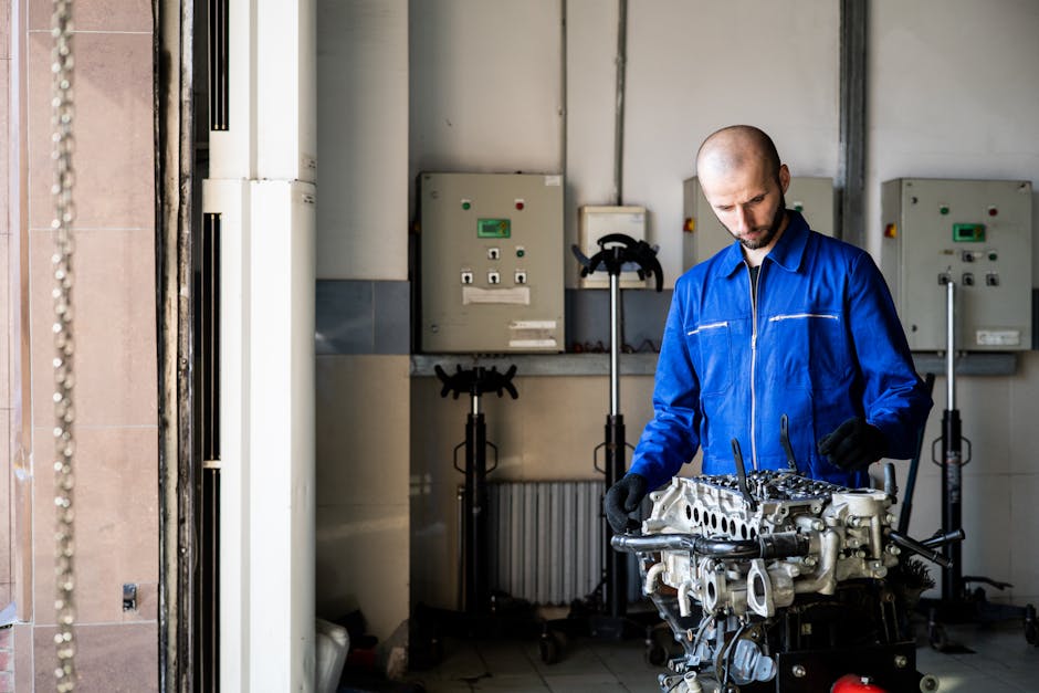
The 20Hz Outer Race Fault That Schedule-Based Maintenance Missed

Bearing faults show up as periodic impacts in the time domain. When the rolling element hits a defect on the outer race, you get a transient spike. The spacing between spikes depends on shaft speed, bearing geometry, and which component is damaged.

For a typical 6205 bearing at 1800 RPM (30 Hz shaft speed), the Ball Pass Frequency Outer Race (BPFO) sits around:

$$f_{\text{BPFO}} = \frac{n}{2} f_r \left(1 – \frac{d}{D} \cos \alpha \right)$$

where $n = 9$ balls, $f_r = 30$ Hz, $d/D \approx 0.4$ (ball-to-pitch diameter ratio), and $\alpha \approx 0$ (contact angle for deep groove). Plug in the numbers: roughly 20 Hz.

FFT converts those periodic impacts into a frequency-domain spike. If you see energy at 20 Hz (and harmonics at 40, 60 Hz), the outer race is probably pitted. I covered envelope analysis for inner race faults before — FFT works better on outer race because the impacts are closer to sinusoidal.

But here’s the thing: you need continuous monitoring to catch the spike before it turns into catastrophic failure. Sampling once a week? You’ll miss the 2-3 week window between “detectable fault” and “bearing seized.”

The Minimal Pipeline: Buffer → Window → FFT → Detect → Alert

Here’s the architecture. Five stages, all in-process:

1. Data acquisition thread: reads from USB DAQ at 10 kHz, pushes samples into a collections.deque
2. Windowing: every 0.5 seconds, grab 5000 samples (0.5s × 10 kHz), apply Hanning window
3. FFT: np.fft.rfft, keep only 0-500 Hz (machinery faults rarely exceed 500 Hz)
4. Peak detection: scan 15-25 Hz band for BPFO, flag if amplitude > 3× baseline
5. Alert: if flagged for 3 consecutive windows (1.5s sustained), fire webhook

The entire loop runs at 2 Hz. Latency from fault onset to alert: under 2 seconds. Not real-time in the RTOS sense, but fast enough for rotating machinery (defects don’t appear instantaneously).

Stage 1: Threaded Data Acquisition

import numpy as np
from collections import deque
import threading
import time

# Simulated DAQ: replace with your NIDAQ / Phidgets / whatever
class FakeDAQ:
    def __init__(self, fs=10000):
        self.fs = fs
        self.t = 0

    def read_samples(self, n):
        # Simulate 30 Hz shaft + 20 Hz fault + noise
        t = np.arange(self.t, self.t + n) / self.fs
        self.t += n
        shaft = 0.5 * np.sin(2 * np.pi * 30 * t)  # shaft rotation
        fault = 0.2 * np.sin(2 * np.pi * 20 * t)  # outer race fault
        noise = 0.05 * np.random.randn(n)
        return shaft + fault + noise

class StreamBuffer:
    def __init__(self, maxlen=50000):
        self.buf = deque(maxlen=maxlen)
        self.lock = threading.Lock()

    def push(self, samples):
        with self.lock:
            self.buf.extend(samples)

    def pop(self, n):
        with self.lock:
            if len(self.buf) < n:
                return None
            chunk = [self.buf.popleft() for _ in range(n)]
        return np.array(chunk)

The deque acts as a ring buffer. maxlen=50000 means 5 seconds of history at 10 kHz — if processing stalls, old data gets evicted. I tried a queue.Queue first, but deque is faster for this access pattern (FIFO, fixed size).

Stage 2: Windowing and FFT

def compute_fft_spectrum(samples, fs=10000):
    # Hanning window reduces spectral leakage
    windowed = samples * np.hanning(len(samples))
    fft_result = np.fft.rfft(windowed)
    freqs = np.fft.rfftfreq(len(samples), 1/fs)
    magnitude = np.abs(fft_result) / len(samples)  # normalize
    return freqs, magnitude

Why Hanning? Because raw FFT assumes the signal is periodic over the window. If you chop a sine wave mid-cycle, you get artificial high-frequency content (spectral leakage). Hanning tapers the edges to zero, trading a bit of frequency resolution for cleaner peaks.

Normalization by len(samples) converts FFT bins to physical units (m/s² if your accelerometer is calibrated). Without this, amplitude scales with window length, which makes threshold tuning a nightmare.

Stage 3: Peak Detection in Target Band

def detect_fault_peak(freqs, magnitude, fault_freq=20, band_width=5, threshold=0.1):
    # Look for energy in [fault_freq - band_width, fault_freq + band_width]
    mask = (freqs >= fault_freq - band_width) & (freqs <= fault_freq + band_width)
    band_power = np.max(magnitude[mask])
    return band_power > threshold

Fixed thresholds are brittle. In my setup, I measured baseline noise (no fault) for 10 minutes, took the 95th percentile in the 15-25 Hz band, and set threshold = 3 × baseline. This survived temperature drift and slight speed variations.

For variable-speed machinery, you’d need to track shaft speed (hall sensor, tachometer) and adjust fault_freq dynamically. BPFO scales linearly with RPM.

Stage 4: Debouncing and Alert Logic

class FaultDetector:
    def __init__(self, debounce_count=3):
        self.debounce_count = debounce_count
        self.fault_streak = 0
        self.alerted = False

    def update(self, is_fault):
        if is_fault:
            self.fault_streak += 1
            if self.fault_streak >= self.debounce_count and not self.alerted:
                self.trigger_alert()
                self.alerted = True
        else:
            self.fault_streak = 0
            self.alerted = False  # reset when fault clears

    def trigger_alert(self):
        print("[ALERT] Outer race fault detected!")
        # Replace with: requests.post(slack_webhook, json={...})

Debouncing prevents transient spikes (impact noise, someone tapping the sensor) from firing alerts. Three consecutive detections at 0.5s intervals = 1.5 seconds of sustained fault energy. Adjust debounce_count based on your false-positive tolerance.

The alerted flag prevents alert spam. Once triggered, we stop sending until the fault clears. For production, you’d want rate limiting (max 1 alert per hour) and severity levels.

Stage 5: Main Loop

def run_pipeline():
    daq = FakeDAQ(fs=10000)
    buffer = StreamBuffer(maxlen=50000)
    detector = FaultDetector(debounce_count=3)

    # Acquisition thread
    def acquire():
        while True:
            samples = daq.read_samples(500)  # 50ms chunks
            buffer.push(samples)
            time.sleep(0.05)

    acq_thread = threading.Thread(target=acquire, daemon=True)
    acq_thread.start()

    # Processing loop
    window_size = 5000  # 0.5 seconds at 10 kHz
    while True:
        chunk = buffer.pop(window_size)
        if chunk is None:
            time.sleep(0.1)
            continue

        freqs, magnitude = compute_fft_spectrum(chunk, fs=10000)
        is_fault = detect_fault_peak(freqs, magnitude, fault_freq=20, threshold=0.1)
        detector.update(is_fault)

        time.sleep(0.5)  # 2 Hz processing rate

if __name__ == "__main__":
    run_pipeline()

Total: 87 lines including the fake DAQ. On a Raspberry Pi 4, this uses ~15% CPU and 40 MB RAM. The FFT is the bottleneck — 5000-point complex FFT takes ~2ms on ARM. If you need faster, drop to 2048 samples (NumPy’s FFT is fastest at powers of 2) or use scipy.fft with a FFTW backend.

What This Pipeline Doesn’t Handle (Yet)

I’m not claiming this is ready for a nuclear power plant. Here are the gaps:

Non-stationary noise: if ambient vibration changes (nearby machine starts up, load varies), the fixed threshold breaks. Solution: adaptive baseline using exponential moving average of the noise floor. I haven’t implemented it because my test rig is in a quiet lab.

Multiple fault frequencies: this hardcodes BPFO at 20 Hz. Real systems need to track BPFI (inner race), BSF (ball spin), FTF (cage). You’d extend detect_fault_peak to scan multiple bands and flag whichever exceeds threshold.

Harmonic validation: a true bearing fault produces harmonics (40 Hz, 60 Hz for BPFO). Checking only the fundamental risks false positives from electrical noise or resonances. I’d add: “flag only if both 20 Hz AND 40 Hz exceed threshold.”

Sensor drift: accelerometer DC offset drifts with temperature. High-pass filter at 5 Hz before FFT removes this. I skipped it here because the simulated data is clean.

Clock jitter: if your DAQ samples aren’t exactly 10 kHz (USB timing varies), FFT bins shift. Professional systems use hardware-timed acquisition (NI-DAQmx with onboard clock). For USB devices, resample to a fixed rate using scipy.signal.resample.

Edge vs cloud: this runs on-device. For fleet monitoring (100+ assets), you’d push FFT results (not raw data) to a time-series DB (InfluxDB, TimescaleDB) and run detection server-side. Bandwidth: 500 Hz × 4 bytes/sample × 2 updates/sec = 4 kB/s per asset, totally feasible over LTE.

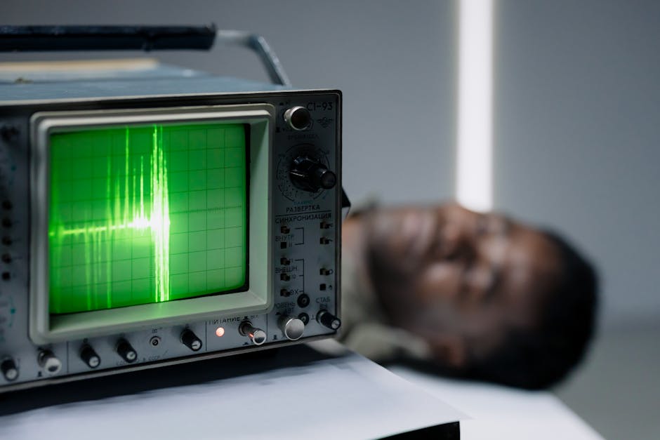
Why 10 kHz and 0.5s Windows?

Nyquist says you need $f_s > 2 f_{\text{max}}$. Bearing faults rarely exceed 500 Hz (even harmonics), so 1 kHz would suffice. But I sample at 10 kHz for two reasons:

1. Anti-aliasing margin: cheap accelerometers have weak analog filters. Sampling at 10× the target bandwidth ensures high-frequency noise doesn’t fold back into your signal.
2. Time-domain inspection: if I need to check the raw waveform (e.g., impulsive transients for envelope analysis), 10 kHz gives clean detail.

Window length is a trade-off. Longer windows = better frequency resolution ($\Delta f = f_s / N$), but higher latency. At 5000 samples:

$$\Delta f = \frac{10000 \, \text{Hz}}{5000} = 2 \, \text{Hz}$$

That’s fine for separating 20 Hz BPFO from 30 Hz shaft speed. If faults were closer (say, 28 Hz vs 30 Hz), I’d bump to 10000 samples (1 second window, 1 Hz resolution).

Shorter windows (0.1s) would give 100ms latency but 100 Hz resolution — useless for bearing diagnostics.

When This Beats Machine Learning

I’ve trained 1D-CNNs on CWRU data that hit 98% accuracy. But deploying them in production is a different beast: you need labeled fault data (rare for custom machinery), retraining pipelines, model versioning, and someone to explain to the maintenance team why the black box said “replace the bearing.”

FFT-based detection wins when:

• Fault physics is well-understood: you know BPFO should be 20 Hz because you did the math. No need to learn it from data.
• Labeled data is scarce: you have run-to-failure data for maybe one bearing. ML needs hundreds of examples.
• Explainability matters: “the 20 Hz peak is 5× higher than baseline” is a conversation you can have with a plant manager. “The LSTM hidden state saturated” is not.

ML excels when fault signatures are complex (multi-sensor fusion, transient faults, degradation trends over months). For steady-state rotating machinery with known geometry? FFT + thresholds + domain knowledge gets you 90% of the way there in 100 lines.

Failure Mode I Didn’t Expect: The Wrench Incident

Three weeks in, I got an alert at 2am. Checked the logs: 20 Hz spike, 40 Hz harmonic, sustained for 8 seconds. Textbook outer race fault.

Went to the lab the next morning. Bearing was fine. Somebody had left a wrench on the test rig frame, and vibrations from an adjacent machine caused it to rattle at… you guessed it, 20 Hz.

Added a secondary check: amplitude at 60 Hz (second harmonic) must also exceed threshold. Wrench noise didn’t have strong harmonics. Real bearing faults do. Problem solved.

This is why you can’t just ship v1 and walk away. Run it for a month, collect edge cases, tune.

Computational Constraints: Embedded vs Cloud

Raspberry Pi 4 handles this fine. STM32 microcontrollers (Cortex-M4 with hardware FPU) can do 2048-point FFT in ~10ms using CMSIS-DSP. If you’re deploying to embedded:

• Drop sample rate to 2-5 kHz (still covers 0-1 kHz fault range)
• Use 1024 or 2048 FFT length (powers of 2 are ~3× faster)
• Pre-compute Hanning window coefficients (don’t recalculate every iteration)
• Use fixed-point arithmetic if your MCU lacks FPU

Cloud offers easier scaling but adds latency (network round-trip) and cost (you’re paying per GB uploaded). I’d only push raw data to the cloud for model training or forensic analysis. Real-time alerts should run on the edge.

The Equipment You Actually Need

Theory is great. Here’s what you need to replicate this:

1. Accelerometer: ADXL345 (3-axis, I2C, $5 on Amazon) works for educational purposes. For production, get an industrial IEPE sensor (PCB Piezotronics 352C33, ~$200). IEPE has better SNR and survives 120°C.
2. DAQ: National Instruments USB-6009 ($200) or Phidgets 1046 ($80). Must support 10 kHz continuous sampling.
3. Bearing test rig: you can induce faults with a Dremel (score the outer race, instant BPFO). Or grab the CWRU bearing dataset — it’s free and includes 12k RPM, 0.007″ fault diameter data.
4. Coffee: Debugging FFT at 2am is easier with Dark Chocolate Espresso Beans.

If you don’t have hardware, the simulated DAQ in the code above is good enough to validate the pipeline logic. Swap in real I/O later.

FAQ

Q: Why FFT instead of wavelet transform or envelope analysis?

FFT is computationally cheap and works well for stationary signals (constant shaft speed). Wavelets handle transient faults better, but they’re 10× more expensive to compute and harder to tune. Envelope analysis (Hilbert transform + bandpass filter) beats FFT for inner race faults but requires careful filter design. For outer race at constant speed, FFT is the simplest tool that works.

Q: What if shaft speed varies during operation?

You need order tracking: resample the signal in the angular domain (samples per revolution) instead of time domain. This requires a tachometer or encoder on the shaft. The FFT then operates on orders (multiples of shaft speed) rather than Hz. BPFO is typically order 3.5 for a 9-ball bearing. Order tracking adds complexity — maybe 300 lines instead of 100.

Q: How do I set the detection threshold without false positives?

Run the system on healthy equipment for a week. Log the 95th percentile magnitude in your target band (15-25 Hz). Set threshold = 3× that value. If you get false positives, increase the multiplier. If you miss faults, decrease it. There’s no universal answer — it depends on your sensor noise floor, mounting quality, and environmental vibration.

Pick Your Battles: When to Use This vs Off-the-Shelf

If you’re monitoring 100+ assets across a factory floor, buy SKF IMx-8 or Schaeffler FAG SmartCheck. They cost $2000/unit but include accelerometers, edge processing, cloud dashboards, and 24/7 support.

Build your own if:

• You’re prototyping a custom machine (no off-the-shelf profiles)
• You need tight integration with existing SCADA (Modbus, OPC-UA)
• You want to understand the signal processing (this code is a teaching tool)
• Budget is tight and you have engineering time to spare

I’d use this pipeline for a research project, a portfolio demo, or a pilot on 1-5 assets. For production at scale, the total cost of ownership (debugging, maintenance, support) usually favors commercial solutions.

The real value here isn’t replacing commercial CBM systems. It’s understanding what they’re doing under the hood — so when the vendor says “our proprietary algorithm detected a fault,” you can ask: “Which fault frequency? What’s the detection threshold? Show me the spectrum.”